From an image to radial profiles

Step 1

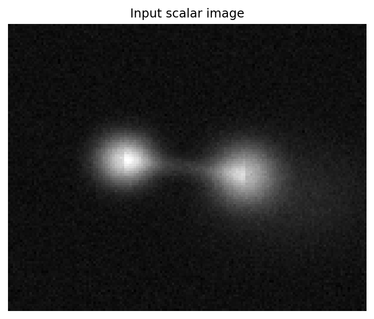
Inspect the scalar image

The example contains two compact peaks, a faint bridge, an asymmetric outer envelope, and a fixed realization of Gaussian background noise. The image is two-dimensional and the PSF FWHM is specified in pixels.

Synthetic astronomical scalar image with two compact peaks and a bridge — The deterministic input image used by the executed notebook.

Step 2

Estimate the background and smooth at the PSF scale

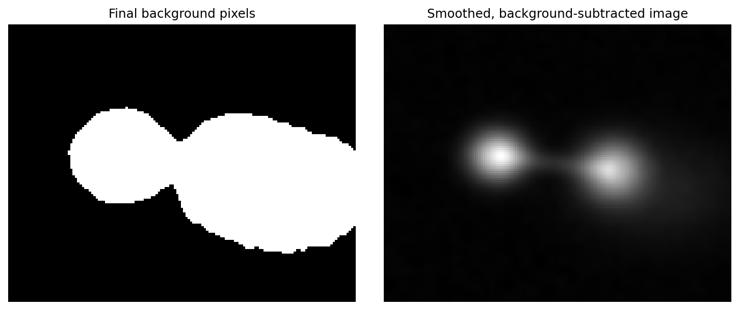
The paper preset starts with the outer 20 per cent border, estimates the background with the median and 1.4826 MAD, and iteratively excludes provisional source pixels. It reports the final background mask, background level, scatter, and number of iterations.

background = estimate_background(
    image, error=error, psf_fwhm=4.0, preset="paper"
)
support_stage = prepare_support(
    image,
    background=background.background,
    sigma_bg=background.sigma_bg,
    psf_fwhm=4.0,
    preset="paper",
)

Final background pixels and smoothed background-subtracted image — The returned mask makes the background estimate inspectable.

Step 3

Construct the provisional support

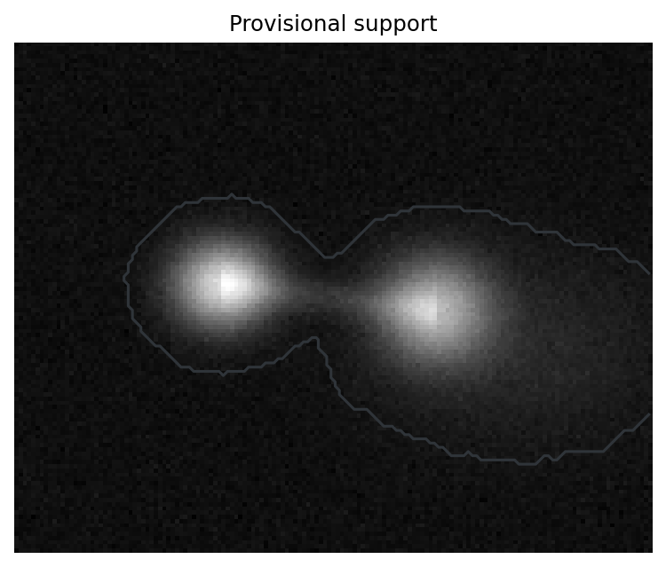
Pixels at or above the smoothed 1.5-sigma threshold are closed and dilated with PSF-scaled circular footprints. Internal holes are not filled. Connected-component selection is postponed until supplied centres are known.

Input image with the provisional support outlined — The outline encloses every provisional connected component retained at this stage.

Step 4

Review centre candidates

Local maxima above five background sigmas are collapsed by connected plateau and ranked by smoothed intensity. The numbered overlay and table persist the coordinates and ranking used for selection.

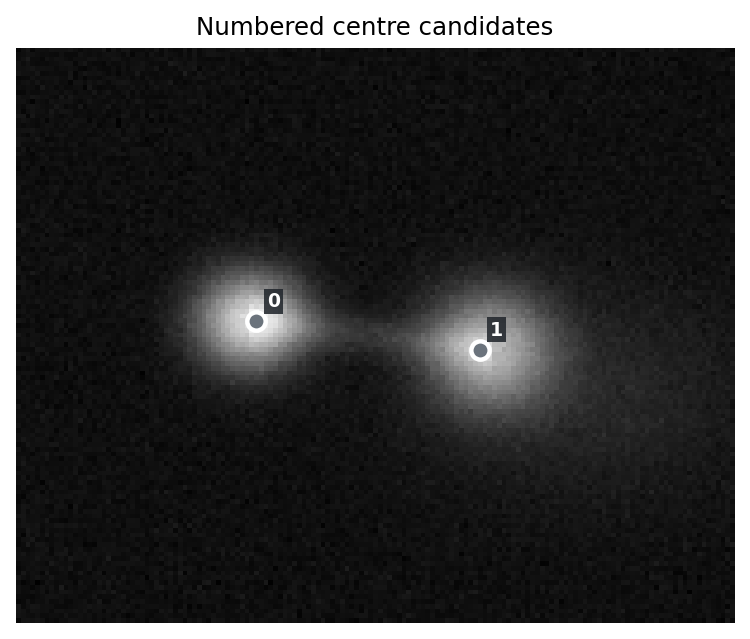
Image with two numbered candidate-centre markers — Candidate numbers correspond to zero-based rows in the table.

candidate	x	y	smoothed peak	significance
0	50	57	1.00966	53.26
1	97	63	0.87037	45.89

Step 5

Select the supplied centres

The example selects candidates [0, 1]. An analysis may select other candidate indices or bypass candidate detection with centres measured independently. Centre count is therefore an explicit user decision.

selected = [0, 1]
centres = select_centres(candidates, indices=selected)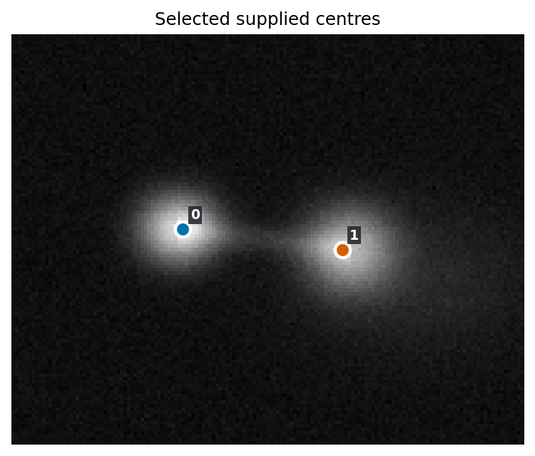

Image with the two selected supplied centres — Selected centres retain the same numbers used during candidate review.

Step 6

Retain the connected support containing every centre

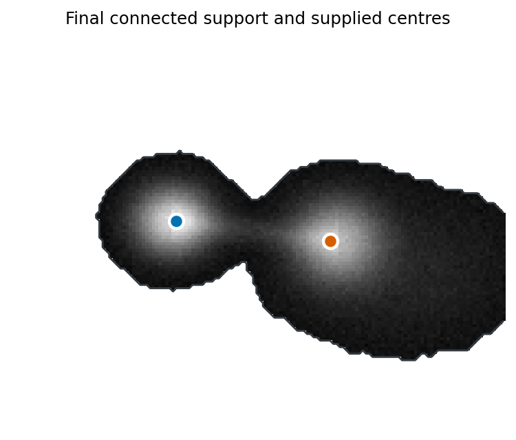
The final support is the one 8-connected provisional component that contains all supplied centres. If selected centres lie in different components, the function raises an error; it does not join components or silently discard a centre.

final = finalize_support(
    support_stage.provisional_support, centres, connectivity=8
)

Final connected support with two supplied centres — The mask and supplied centres now form the complete geometry input.

Step 7

Build both radial coordinates

build_geometry receives only the final support and supplied centres. It does not repeat image preparation or infer new centres. The public result stores its distance and coordinate arrays in float64 precision.

geometry = build_geometry(final.support, centres)

rho_d = geometry.rho_D
rho_x = geometry.rho_X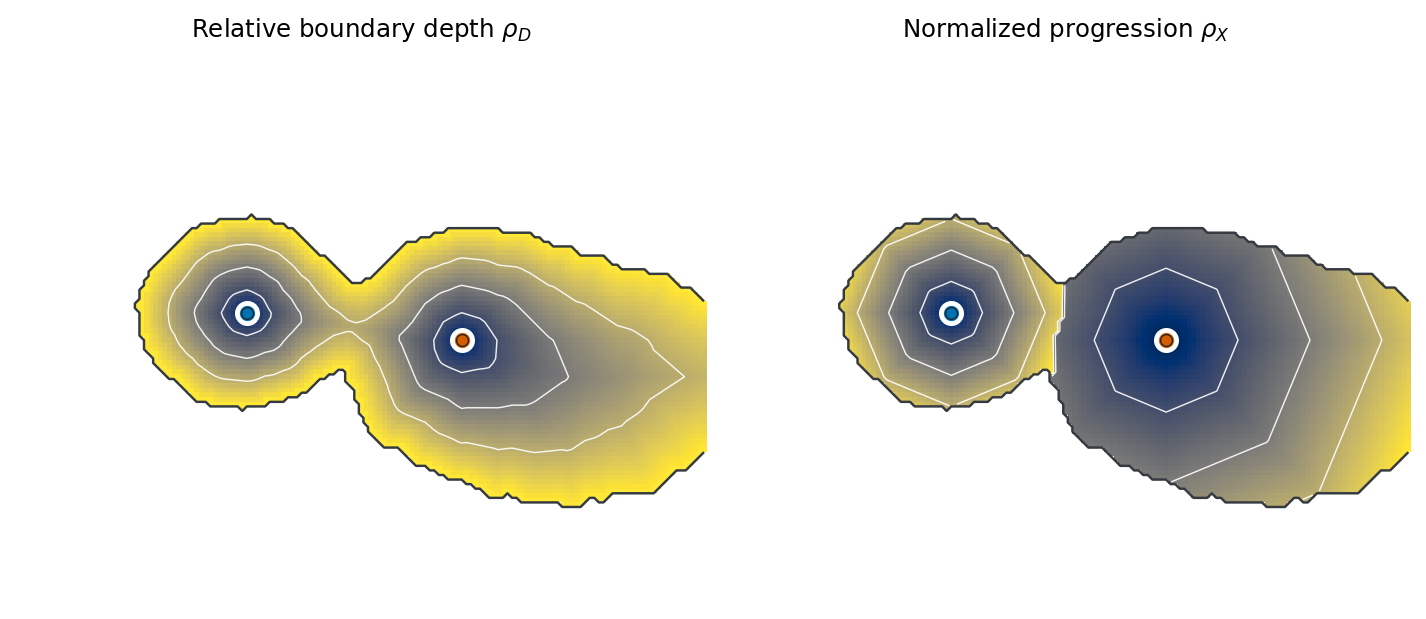

Relative centre-boundary depth and normalized progression coordinate maps — Relative centre–boundary depth (left) and normalized progression (right) are constructed on the same support.

Step 8

Measure a registered tracer

Geometry is reusable. A registered intensity, colour, velocity, age, or metallicity image can be summarized without changing the support, centre assignment, or radial coordinates.

brightness = radial_profile(image, geometry, coordinate="rho_D")
progression = radial_profile(image, geometry, coordinate="rho_X")

The default estimator uses 30 equal bins on [0, 1], includes ρ = 1 in the final bin, omits bins with fewer than six pixels, and reports the unweighted median in each centre-associated region.

Focused examples

Continue with the notebooks

Each notebook has one purpose and can be downloaded independently.

01 · Quick startSupport, centres, geometry, and one profile 02 · Understanding coordinatesInternal boundaries and coordinate interpretation 03 · Your own imageThe complete preprocessing tutorial shown above 04 · Registered tracersReuse one geometry across several scalar fields