Sagui prepares a common multiband cube, constructs a spatial support, assigns categorical regions, and measures their integrated SEDs.
Install
install.packages("remotes")
remotes::install_github("RafaelSdeSouza/sagui", upgrade = "never")
library(sagui)
Simulate a galaxy
This fixed-seed simulation mixes bulge, disc, and two knot profiles in nine bands.
set.seed(42)
bands <- c(0.90, 1.15, 1.50, 1.82, 2.00, 2.77, 3.56, 4.10, 4.44)
nx <- ny <- 24L
xy <- expand.grid(x = seq_len(nx), y = seq_len(ny))
dx <- xy$x - 12.5
dy <- xy$y - 12.5
radius <- sqrt((dx / 1.10)^2 + (dy / 0.78)^2)
support <- matrix((dx / 11)^2 + (dy / 8.3)^2 <= 1, nx, ny)

profiles <- rbind(
  bulge = c(0.58, 0.78, 1.02, 1.16, 1.14, 0.98, 0.82, 0.72, 0.66),
  disc  = c(0.82, 0.94, 1.04, 1.08, 1.05, 0.92, 0.84, 0.78, 0.74),
  knot1 = c(1.18, 1.11, 1.02, 0.96, 0.93, 0.88, 0.98, 0.91, 0.86),
  knot2 = c(1.08, 1.04, 0.99, 0.95, 0.94, 0.91, 1.05, 0.99, 0.93)
)
weights <- cbind(
  exp(-(radius / 3.0)^2),
  exp(-radius / 8.5),
  exp(-((dx - 4.5)^2 + (dy + 1.8)^2) / 5),
  exp(-((dx + 4.0)^2 + (dy - 2.6)^2) / 6)
)
weights <- weights / rowSums(weights)
brightness <- 0.12 + 1.35 * exp(-radius / 8)
flux <- brightness * (weights %*% profiles)
flux <- flux + matrix(rnorm(length(flux), sd = 0.012), nrow(flux))
cube <- array(flux, c(nx, ny, length(bands)))
for (b in seq_along(bands)) cube[, , b][!support] <- NA_real_
Segment
The simulated galaxy already uses NA outside its
support, so no starlet mask is needed.
seg <- segment_regions(
  cube,
  Ncomp = 6,
  use_starlet_mask = FALSE,
  cluster_pretransform = "none"
)
table(seg$cluster_map, useNA = "ifany")
#>
#>    1    2    3    4    5    6 <NA>
#>  106   94   30   27   13   14  292
Positive integers are categorical identifiers. Their ordering carries
no physical meaning; NA denotes unassigned background.
Measure SEDs
regional <- extract_region_sed(
  cube,
  seg$cluster_map,
  band_values = bands,
  sigma_band = rep(0.012, length(bands))
)
knitr::kable(head(regional$flux_long), digits = 4)| region | band | flux | flux_err | n_eff | lambda | n_pix |
|---|---|---|---|---|---|---|
| 1 | 0.9 | 51.3139 | 0.1235 | 106 | 0.90 | 106 |
| 1 | 1.15 | 57.4866 | 0.1235 | 106 | 1.15 | 106 |
| 1 | 1.5 | 62.6675 | 0.1235 | 106 | 1.50 | 106 |
| 1 | 1.82 | 64.4578 | 0.1235 | 106 | 1.82 | 106 |
| 1 | 2 | 62.8975 | 0.1235 | 106 | 2.00 | 106 |
| 1 | 2.77 | 55.2894 | 0.1235 | 106 | 2.77 | 106 |
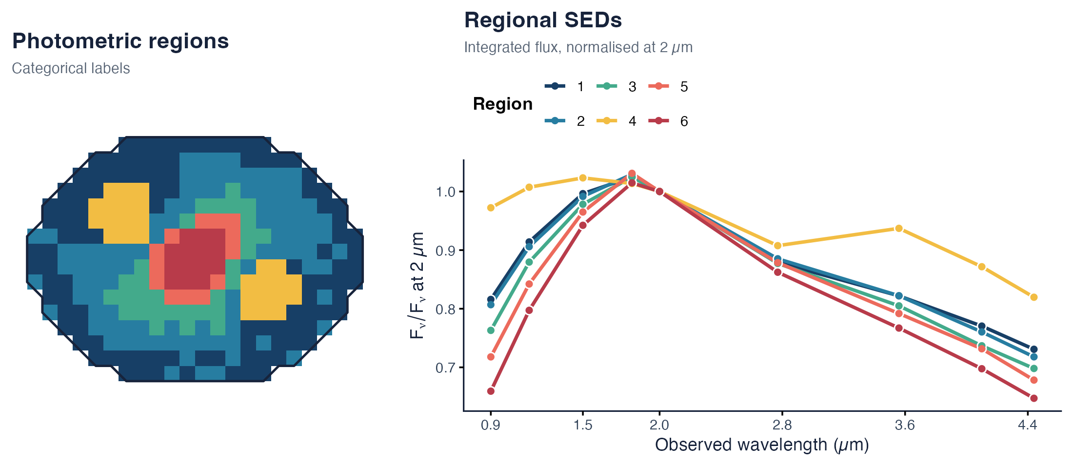
Six categorical regions and their fixed-seed nine-band regional SEDs. Curves are normalised at 2 µm only for shape comparison.
Continue with Prepare Photometry for observations, or Export Regional SEDs to save the results.