
Photometric SED segmentation for resolved galaxies.
Sagui turns a PSF-matched multiband cube into spatially coherent regions and flux-preserving regional spectral energy distributions (SEDs). It supports exact Ward clustering for compact data and sparse-graph Ward clustering for larger images.
The methods and first applications are described by de Souza et al. (2026), sagui: SED-based segmentation of multiband Galaxy images – application to JADES in GOODS-South, arXiv:2604.18812.
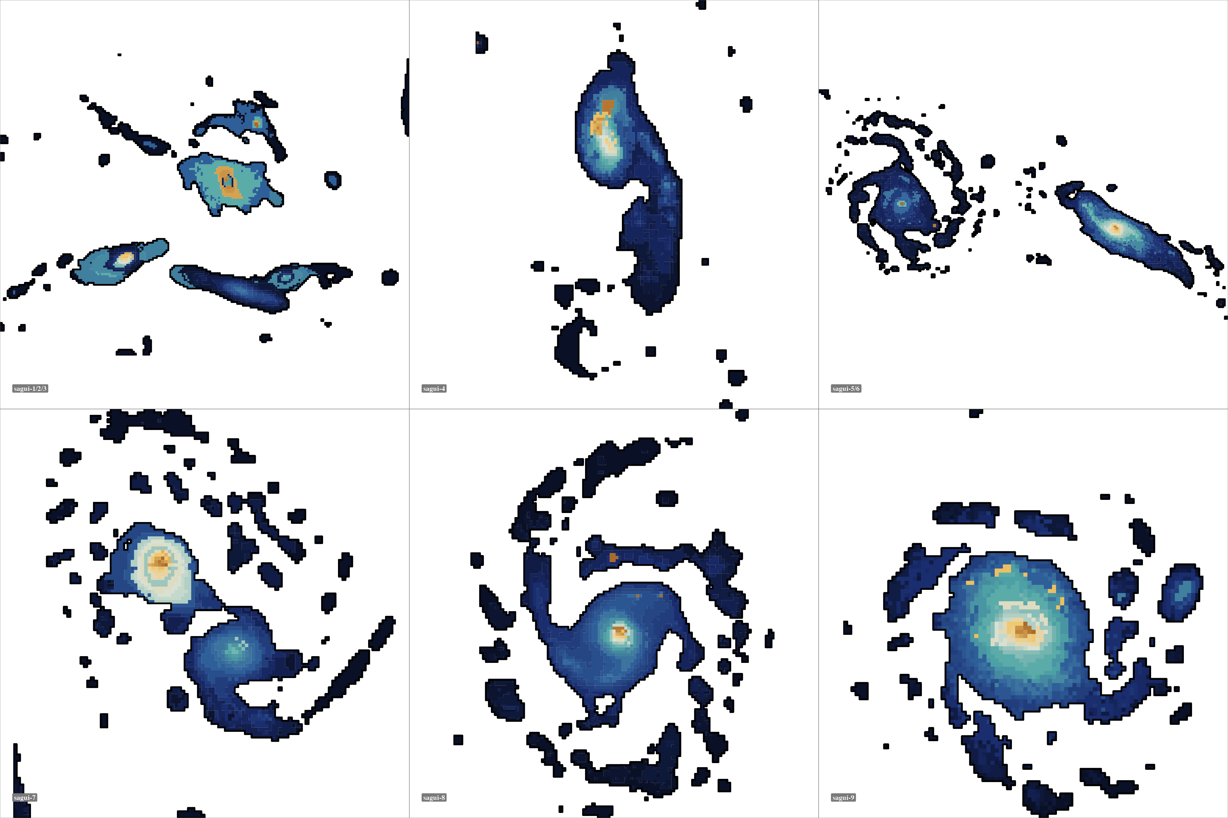
- PrepareAlign the images, match the PSF, and assemble the band axis.
- SupportDefine which pixels belong to the astronomical source.
- SegmentGroup photometric SEDs with exact or sparse Ward clustering.
- MeasureExport regional fluxes and uncertainties for SED fitting.
Install
install.packages("remotes")
remotes::install_github("RafaelSdeSouza/sagui")
library(sagui)
Quick start
This example simulates a small resolved galaxy in nine near-infrared bands. Its pixels mix bulge, disc, and two star-forming-knot SED profiles inside an elliptical support.
set.seed(42)

bands <- c(0.90, 1.15, 1.50, 1.82, 2.00, 2.77, 3.56, 4.10, 4.44)
nx <- ny <- 24L
xy <- expand.grid(x = seq_len(nx), y = seq_len(ny))
dx <- xy$x - 12.5
dy <- xy$y - 12.5
radius <- sqrt((dx / 1.10)^2 + (dy / 0.78)^2)
support <- matrix((dx / 11)^2 + (dy / 8.3)^2 <= 1, nx, ny)

profiles <- rbind(
  bulge = c(0.58, 0.78, 1.02, 1.16, 1.14, 0.98, 0.82, 0.72, 0.66),
  disc  = c(0.82, 0.94, 1.04, 1.08, 1.05, 0.92, 0.84, 0.78, 0.74),
  knot1 = c(1.18, 1.11, 1.02, 0.96, 0.93, 0.88, 0.98, 0.91, 0.86),
  knot2 = c(1.08, 1.04, 0.99, 0.95, 0.94, 0.91, 1.05, 0.99, 0.93)
)

weights <- cbind(
  exp(-(radius / 3.0)^2),
  exp(-radius / 8.5),
  exp(-((dx - 4.5)^2 + (dy + 1.8)^2) / 5),
  exp(-((dx + 4.0)^2 + (dy - 2.6)^2) / 6)
)
weights <- weights / rowSums(weights)
surface_brightness <- 0.12 + 1.35 * exp(-radius / 8)
flux <- surface_brightness * (weights %*% profiles)
flux <- flux + matrix(rnorm(length(flux), sd = 0.012), nrow(flux))
cube <- array(flux, dim = c(nx, ny, length(bands)))
for (b in seq_along(bands)) cube[, , b][!support] <- NA_real_

seg <- segment_regions(
  input = cube,
  Ncomp = 6,
  use_starlet_mask = FALSE,
  cluster_pretransform = "none"
)

regional <- extract_region_sed(
  cube = cube,
  labels = seg$cluster_map,
  band_values = bands,
  sigma_band = rep(0.012, length(bands))
)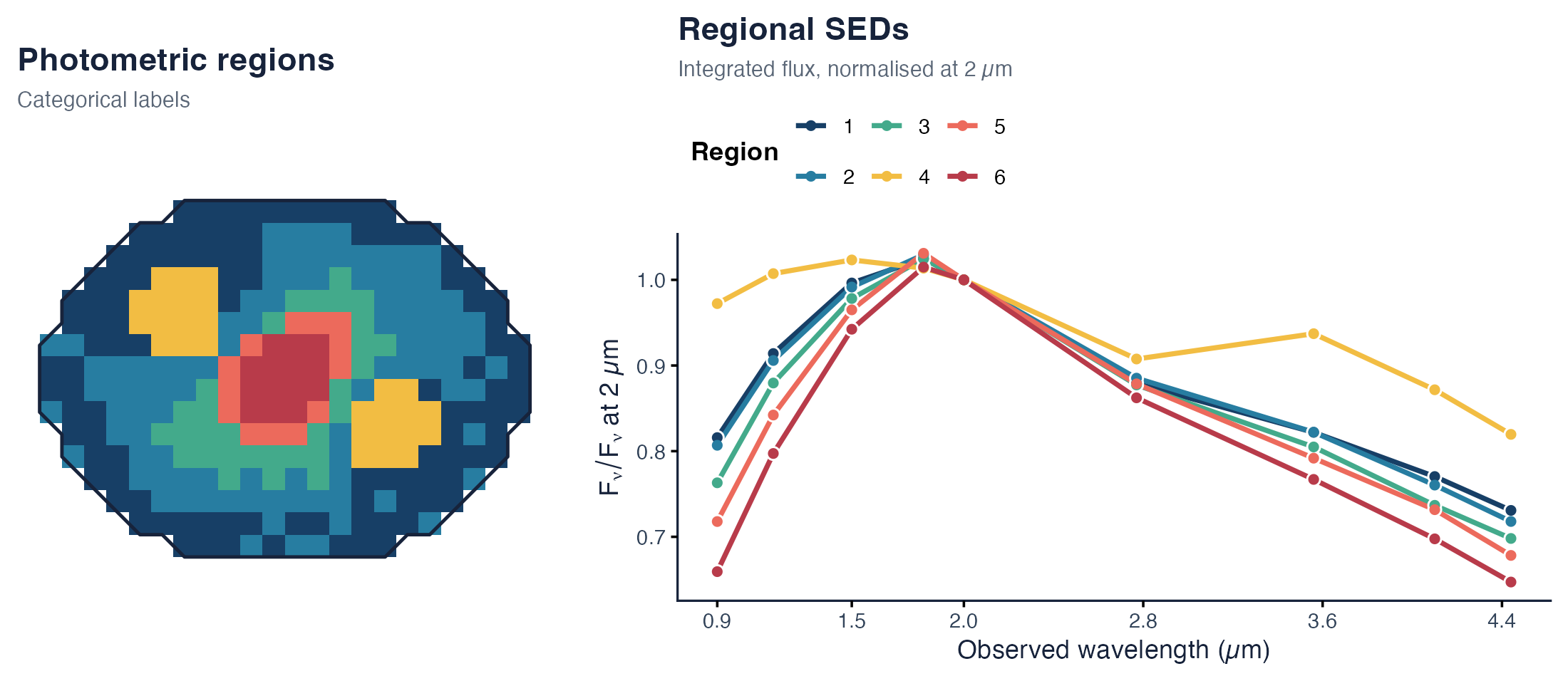
The output contains the integrated photometry for each region:
| region | lambda (µm) | flux | flux error | pixels |
|---|---|---|---|---|
| 1 | 0.90 | 51.3139 | 0.1235 | 106 |
| 1 | 1.15 | 57.4866 | 0.1235 | 106 |
| 1 | 1.50 | 62.6675 | 0.1235 | 106 |
Core API
Use segment_regions() for exact Ward clustering and segment_regions_large() when the all-pairs distance matrix is too large. Both return the categorical region map and the parameters used for the segmentation.
About
Sagui is part of the COIN Toolbox. Please cite the software paper with citation("sagui").